Core Concepts
How Clad Works
Clad is an open source clang plugin that enables automatic differentiation of mathematical functions in C++. Clad which is based on the LLVM compiler infrastructure does this by parsing and transforming the abstract syntax tree (AST); it detects mathematical function and consequently inserts the derived function in the AST.
Forward and Reverse Mode Automatic Differentiation
Forward Mode Automatic Differentiation
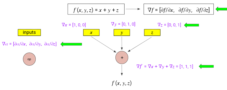
In forward mode AD, one first fixes the independent variable with respect to which differentiation is performed and computes the derivative of each sub-expression recursively. Compared to reverse mode AD, forward mode is natural and easy to implement as the flow of derivative information coincides with the order of evaluation of the mathematical function.
Consider the following equation :
Consider,
Differentiating this eqn w.r.t to any arbitrary variable t we get :
The above equations were obtained using the chain rule for differentiation which is as follows :
\[\pdv{w}{t} = \pdv{w}{u1} * \pdv{u1}{t} + \pdv{w}{u2} * \pdv{u2}{t} ....\]
Here w denotes the output variable and u1 and u2 denote the input variables.
Replacing \(\pdv{a}{t}\) with \(da\) and so on we get.
If we substitute \(t = x\) i.e. we need to substitute \(dx = 1\) and \(dy = 0\). Thus \(dz\) will be \(\pdv{z}{x}\). Similarly we need to substitute \(dy = 1\) as the seed value while differentiating w.r.t \(y\). The disadvantage of the forward mode AD is clearly visible here; we need to calculate derivative w.r.t to both independent variables separately.
Reverse Mode Automatic Differentiation
In reverse mode AD, the dependent variable to be differentiated is fixed and the derivative is computed with respect to each sub-expression recursively. Reverse accumulation traverses the chain rule from outside to inside, or in the case of the directed acyclic graph of the function(often used to show flow of information), from top to bottom. The reverse mode AD requires only one sweep of the computation graph; this is faster than forward mode AD; however it should also be noted that the intermidiate variables need to be stored during computation which may result in significant amount of memory if the computation graph is large.
Thus the simplicity of the foward mode comes with a big disadvantage we need to seed dx = 0 and dy = 1, run the program and then seed dx = 1 and dy = 0 and run another iteration of the program. The cost of forward mode AD thus scales to o(n) where n is the number of input variables. Thus the cost would be very high; if we want to calculate the gradient of a very complicated function with large number of input variables.
Rewriting the chain rule upside down taking advantage of its symmetry we get :
Here we have reversed the roles of the input and output variables. Here u is some input variable and wi is an output variable dependent on u. s is an intermidiate variable to show change in the position of the derivative.
Here we apply the chain rule for every input variable u as opposed to the forward mode where we applied chain rule for every output variable w.
Applying this modified version of the chain rule on our given equations we get :
Replacing \(\pdv{s}{b}\) by sb and so on.
Substituting s = z we will get sz = 1
Thus we don’t need to run the program twice for each input. However, as mentioned above the only drawback is we need to re-run the program for a different output.
Vectorized Forward Mode Automatic Differentiation
Vectorized Forward Mode Automatic Differentiation is a computational technique that combines two powerful concepts: vectorization and forward mode automatic differentiation. This approach is used to efficiently compute derivatives of functions with respect to multiple input variables by taking advantage of both parallel processing capabilities and the structure of the computation graph.
Working
For computing gradient of a function with an n-dimensional input - forward mode requires n forward passes.
We can do this in a single forward pass, instead of accumulating a single scalar value of derivative with respect to a particular node, we maintain a gradient vector at each node. Although, the strategy is pretty similar, it requires three passes for computing partial derivatives w.r.t. the three scalar inputs of the function.
At each node, we maintain a vector, storing the complete gradient of that node’s output w.r.t.. all the input parameters. All operations are now vector operations, for example, applying the sum rule will result in the addition of vectors. Initialization for input nodes are done using one-hot vectors.
Vectorized Forward Mode Automatic Differentiation to compute the gradient.
Benefits
We know that each node requires computing a vector, which requires more memory and more time, which adds to these memory allocation calls. This must be offset by some improvement in computing efficiency.
This can prevent the recomputation of some expensive functions, which would have executed in a non-vectorized version due to multiple forward passes. This approach can take advantage of the hardware’s vectorization and parallelization capabilities using SIMD techniques.
Derived Function Types and Derivative Types
Todo
todo
Custom Derivatives
Todo
todo
Pushforward and Pullback functions
Pushforward functions
Pushforward function of a function computes the output variables sensitivities from the input values and the input variables sensitivities. Intuitively, pushforward functions propagates the derivatives forward. Pushforward functions are constructed by applying the core principles of the forward mode automatic differentiation.
As a user, you need to understand how pushforward function mechanism works so that you can define custom derivative pushforward functions as require and can thus, unlock full potential of Clad.
Mathematically, if a function fn is represented as:
then the corresponding pushforward will be defined as follows:
Here, \(\dot{u} = \pdv{u}{x}\) and \(x\) is the independent variable.
As a concrete example, pushforward of std::sin(double) function will be generated by Clad as follows:
namespace std {
  double sin_pushforward(double x, double d_x) {
    return ::std::cos(x) * d_x;
  }
}
In the forward mode automatic differentiation, we need to compute derivative of each expression in the original source program. Pushforward functions allow to effectively compute and process derivatives of function call expressions. For example:
y = fn(u, v);
In the derived function, this statement will be transformed to:
_d_y = fn_pushforward(u, v, _d_u, _d_v);
y = fn(u, v);
Here, note that:
Here, \(x\) is the independent variable.
From here onwards, in the context of a pushforward function or a usual forward mode derived function, _d_someVar will represent \(\pdv{someVar}{x}\) where \(x\) is the associated independent variable.
Pushforward functions are generated on demand. That is, if Clad needs to differentiate a function call expression, then only it will generate the pushforward of the corresponding function declaration.
For a function:
double fn1(float i, double& j, long double k) { }
the prototype of the corresponding pushforward function will be as follows:
double fn1(float i, double& j, long double k, float _d_i, double& _d_j, long double _d_k);
Please note the following specification of the pushforward functions:
Return type of the pushforward function is same as that of the return type of the source function.
Parameter list of the pushforward function is the parameter list of the original function followed by the parameter list that contains derivative of each differentiable parameter of the source function in the original sequence.
All of these specifications must be exactly satisfied when creating a custom derivative pushforward function.
Pullback functions
Todo
todo
Differentiable Class Types
Todo
todo
Numerical Differentiation
Clad currently provides two interfaces packaged in a single template header file that allows users to easily use numerical differentiation standalone. The two interfaces and their usages are mentioned as follows:
forward_central_difference
The numerical differentiation function that differentiates a multi-argument function with respect to a single argument only. The position of the argument is specified by the user or Clad. This interface is mainly used in Clad’s forward mode for call expressions with single arguments. However, it can also easily be extended for jacobian-vector products. The signature of this method is as follows:
template < typename F, typename T, typename... Args>
  precision forward_central_difference(F f, T arg, std::size_t n, bool printErrors, Args&&... args){
      // Clad has enough type generality that it can accept
      // functions with a variety of input types.
      // Here:
      // f(args...) - is the target function.
      // n - is the position of the parameter with respect to which the derivative is calculated.
      // printErrors - a flag to enable printing of error estimates.
}
central_difference
The numerical differentiation function that differentiates a multi-argument function with respect to all the input arguments. This function returns the partial derivative of the function with respect to every input, and as such is used in Clad’s reverse mode. The signature of the method is as follows:
template <typename F, std::size_t... Ints,
            typename RetType = typename clad::function_traits<F>::return_type,
            typename... Args>
  void central_difference(F f, clad::tape_impl<clad::array_ref<RetType>>& _grad, bool printErrors, Args&&... args) {
      // Similar to the above method, here:
      // f(args...) - is the target function.
      // grad - is a 2D data structure to store all our derivatives as grad[paramPosition][indexPosition]
      // printErrors - a flag to enable printing of error estimates.
}
The above uses functions from the standard math library and so is required to link against the same. To avoid this (and disable numerical differentiation) use -DCLAD_NO_NUM_DIFF at the target program’s compile time.
Implementation Details
Clad uses the five-point stencil method to calculate numerical derivatives. Here, the target function is executed at least 4 times for each input parameter. Since the number of parameters can be different across multiple candidate functions, we use an add-on function to correctly select the parameter whose derivative is to be calculated. The function is described as follows:
// This function enables 'selecting' the correct parameter to update.
// Without this function, Clad will not be able to figure out which x should be updated to x ± h.
template <typename T>
T updateIndexParamValue(T arg, std::size_t idx, std::size_t currIdx, int multiplier, precision& h_val,...) {
    if (idx == currIdx) {
          // selects the correct ith term.
          // assigns it an h_val (h)
          // and returns arg + multiplier * h_val.
    }
    return arg;
  }
Here, Idx is the current parameter and currIdx is the parameter to differentiate with respect to in that pass. If the indices do not match, the argument is returned unchanged.
This function is then applied to all the arguments and is forwarded to the target function f:
fxh = f(updateIndexParamValue(args, indexSeq/*integer index sequence for the parameter pack,
                              Args allows giving an index to each parameter in the pack.*/,
                              i /*index to be differentiated wrt*/,
                              /*±1*/,
                              h/*this is returned*/,
                              /*other params omitted for brevity*/)...);
The above line results in the calculation of f(…, xi ± h, …). Finally the whole algorithm for calculating the gradient of a function (numerically) is as follows:
for each i in args, do:

  fx1 := f(updateIndexParamValue(args, idexSeq, i, 1, h, /*other params*/)...)

  fx2 := f(updateIndexParamValue(args, idexSeq, i, -1, h, /*other params*/)...)

  grad[i][0] := (fx1 - fx2)/(2 * h)

end for
Currently Supported Use Cases
Differentiating multi-arg function calls.
Differentiating calls with pointer/array input.
Differentiating user-defined types.
Printing of error estimates.
Error Estimation Core Concepts
Todo
todo
